Coupling concept
Contents
Coupling concept
One basic problem when dealing with regional climate models system is that the individual components (atmosphere, ocean, land etc.) are described by different models (realized as computer programs) that act on different grids, see Fig. 2 and Fig. 3.
Still, the components have to be coupled in order communicate their state to each other and exchange fluxes as given by nature itself.
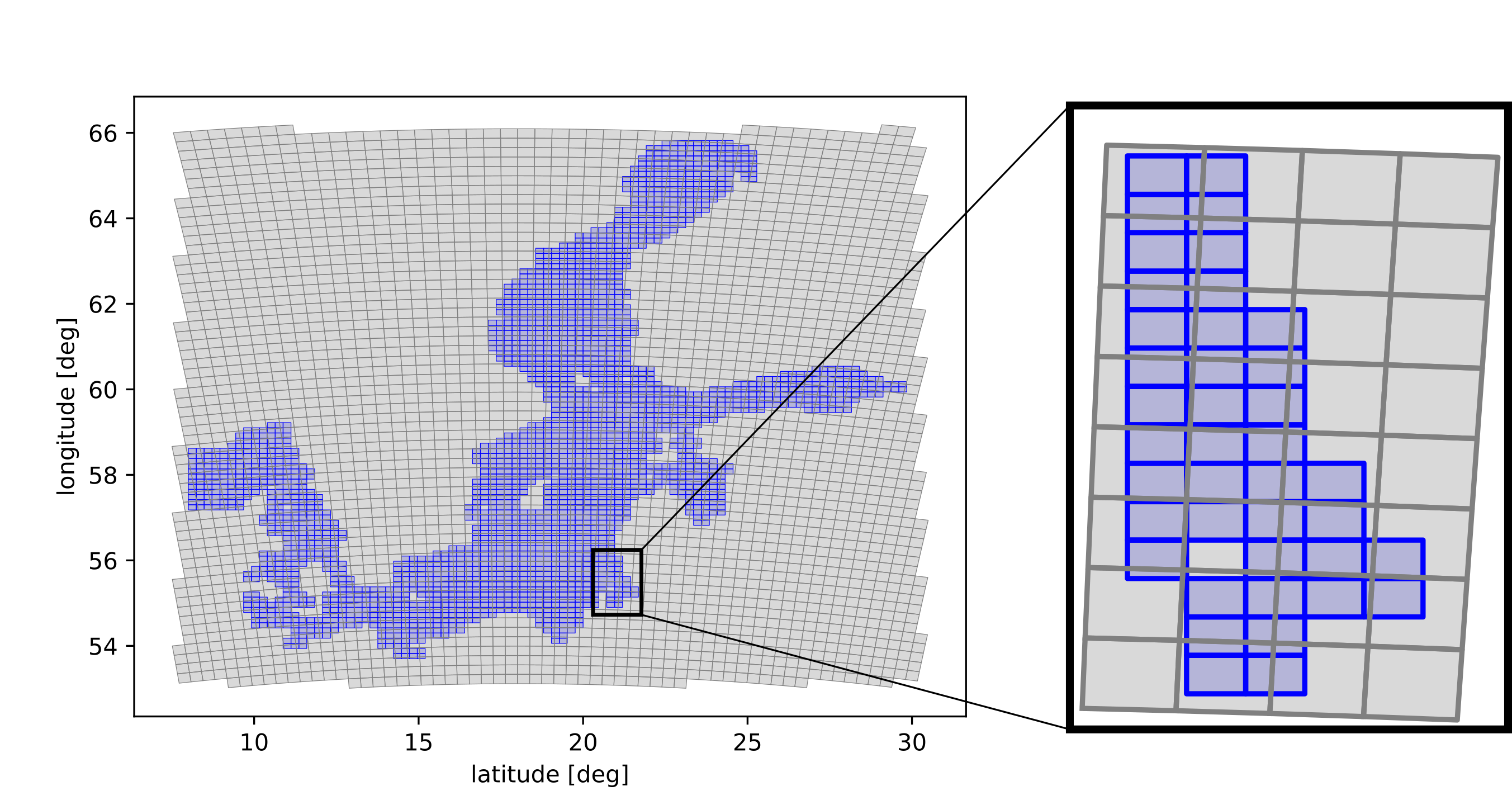
Fig. 2 Overlaying grids of atmospheric and ocean model for the Baltic Sea
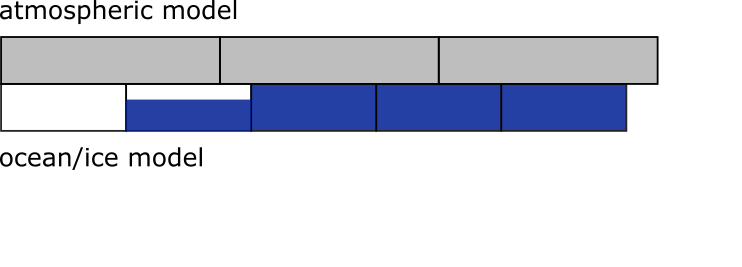
Fig. 3 Abstraction of figure Fig. 2 in one spatial horizontal dimension. Bottom model can support different surface types as water (blue) and ice (white).
To exemplify this problem let us consider the calculation of a flux of something from the atmosphere to the bottom. Usually, if the flux depends on the state of the ocean, some state variables have to be communicated first to the atmosphere. Since the atmospheric grids are normally larger, the information has to be averaged (weighted by areas) over several bottom cells, over different surface types, see Fig. 4.
With this averaged state information and its own internal state, the atmospheric model can now calculate the flux as a field on the atmospheric grid. It is noteworthy that the flux cannot be calculated for the different surface types differently, since the atmospheric model does not know about that (at least not without changing the code significantly). Finally, the flux field then has to be redistributed on the bottom cells (again in a area-weighted manner such that flux variable is overall conserved), see Fig. 5. Since the flux is only calculated from averaged information and not surface-type-dependent, this approach locally not consistent and can become inaccurate. This is especially true if many bottom grid cells are covered by one atmospheric grid cell.
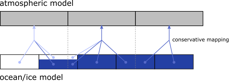
Fig. 4 Average of ocean’s state variables communicated to the atmosphere.
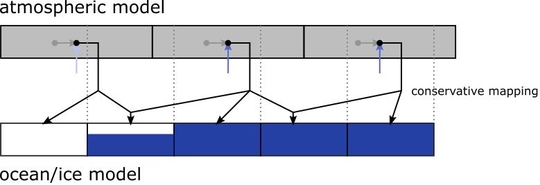
Fig. 5 Calculation of fluxes in the atmospheric model and remapping on to the ocean’s grid.
Current implementation
Available models
At present, the following components can be coupled in the IOW ESM:
COSMO-CLM atmospheric model
MOM5.1 ocean model (including (a) the ERGOM ecosystem model and (b) a dynamic ice model, coupled internally via the FMS coupler)
By its design it is modular, so more models will follow in future that can be interactively coupled together.